Spatial ML · AWS SageMaker · 2026
Lagos Demand Forecasting Engine
A delivery platform cannot react fast enough to demand spikes. By the time a surge is
visible in live orders, it is already too late to position riders. This system predicts where orders will come
in before they arrive, so riders are already there.
The problem it solves
When riders sit idle in quiet zones while high-demand zones are understaffed, customers wait longer, cancel
orders, and switch to competitors. The fix is prediction, not reaction.
How it works
NYC taxi trip data is used as a training proxy. Taxi pickups and food delivery orders are driven by the same
forces: time of day, day of week, and neighbourhood density. Every pickup coordinate is converted into an H3
hexagon — a uniform 500m delivery zone cell. The system counts demand per zone per hour, engineers lag and
rolling average features, and trains a LightGBM model to predict the next hour's demand per zone. The output
tells operations how many riders to pre-stage in each zone.
What was built
- H3 spatial indexing pipeline converting raw coordinates into uniform delivery zone cells
- Feature engineering with lag features (1h, 2h, 3h, 24h, 7-day same hour), rolling averages, and
time-of-day flags
- LightGBM regression model with log-transform on the target to handle demand imbalance across zones
- Full SageMaker pipeline: Processing Job, Training Job, Model Registry, real-time inference endpoint
- Rider allocation output: predicted demand translated directly into staging recommendations
Model improvement
The first model had a test error of 6.95 trips per zone per hour. Two changes were made: a log-transform on
the target variable so high-demand zones stop being treated as outliers, and extended lag features adding
2-hour and 3-hour lookback. Test error dropped to approximately 2.2 real trips per hour — a 68% reduction.
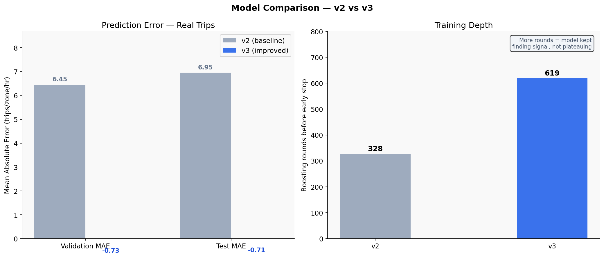
Left: prediction error in real trips per zone per hour. Right: boosting rounds
before early stopping. More rounds means the model kept finding signal rather than plateauing.
Demand analysis
Before training any model, the data was explored to understand what actually drives demand. Four patterns
emerged that directly shaped the feature set.
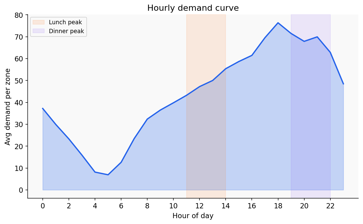
Demand collapses to its lowest point around 4am, then climbs steadily and peaks at
6pm to 7pm. The lunch and dinner windows are flagged as key delivery periods. The model learns this daily
shape as its baseline.
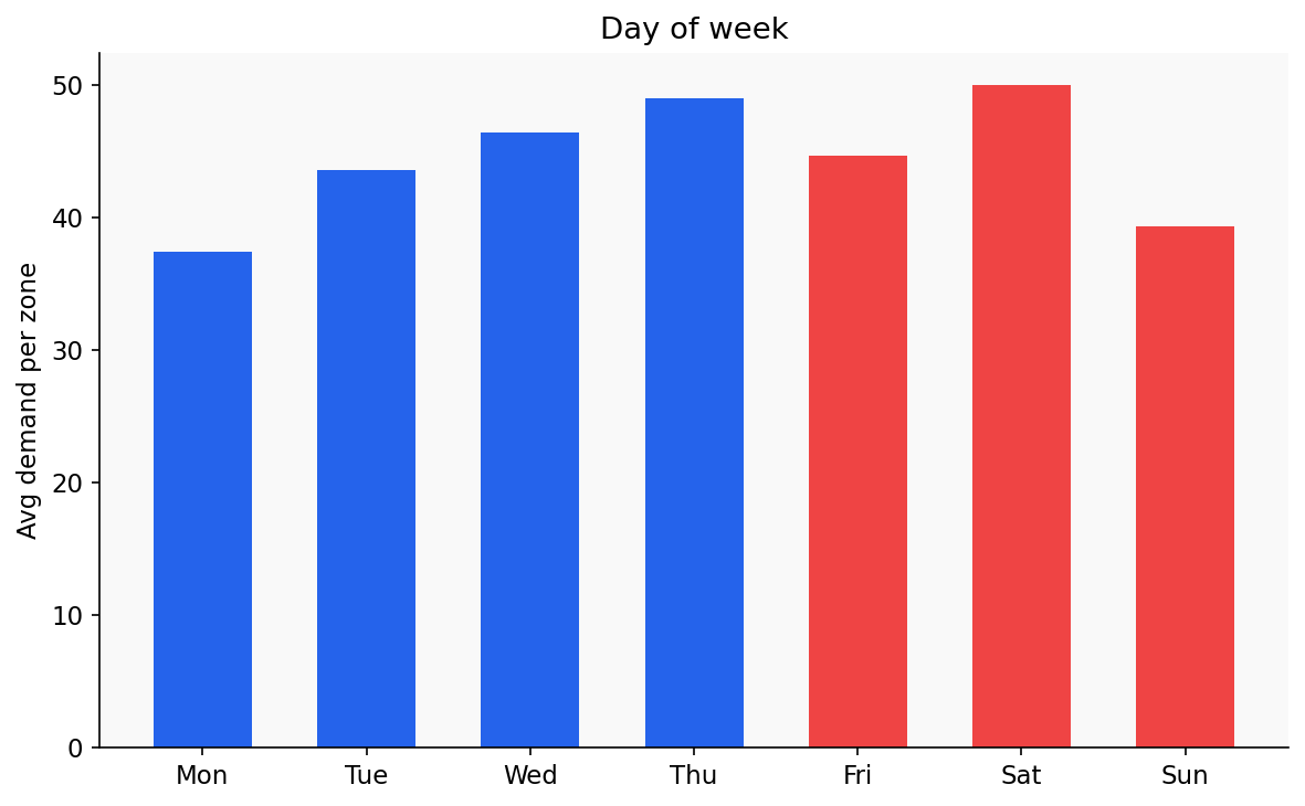
Saturday is the busiest day of the week. Demand builds from Monday, peaks Thursday
and Saturday, then drops Sunday. Rider supply planning should scale through the week, not treat every day
equally.
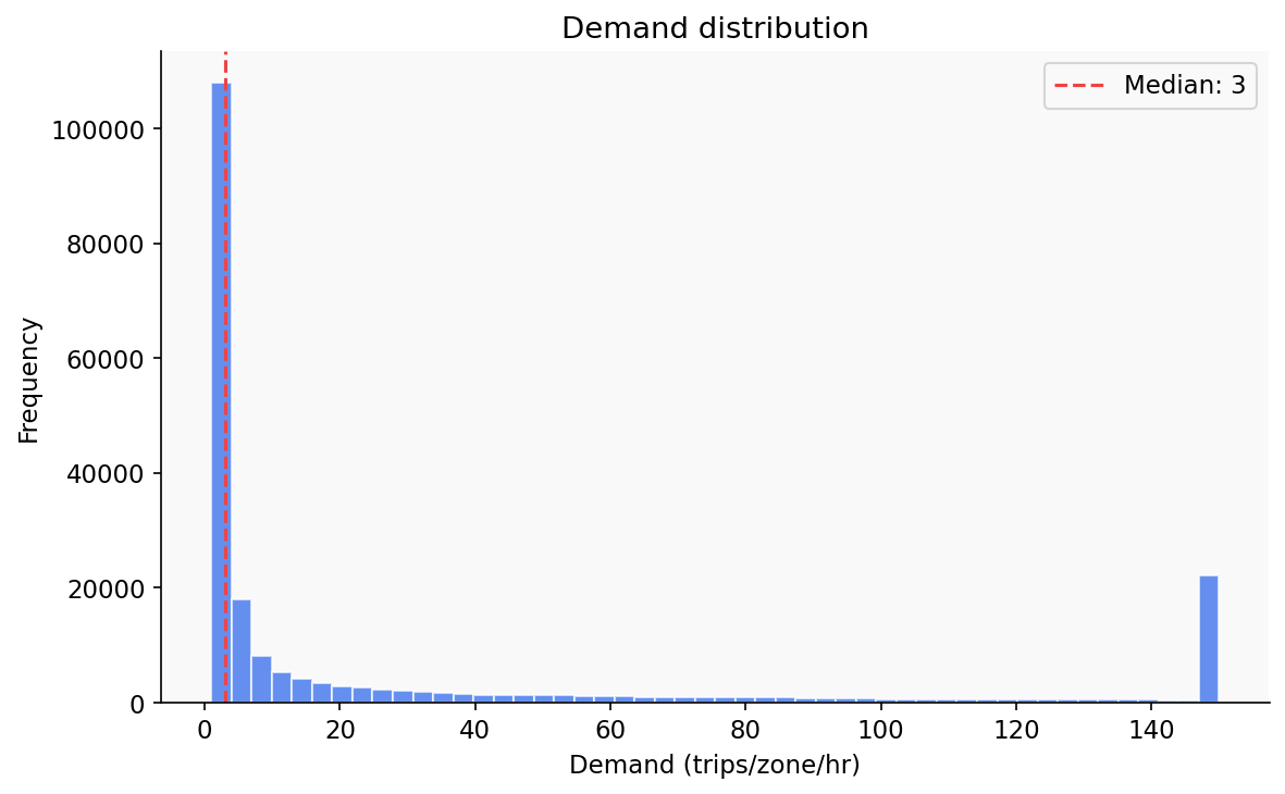
Most zones are quiet most of the time — the median is 3 trips per zone per hour. A
small number of hot zones handle over 100 trips per hour. This is exactly why the log-transform matters:
without it, the model spends all its learning on quiet zones and ignores the ones that actually drive
revenue.
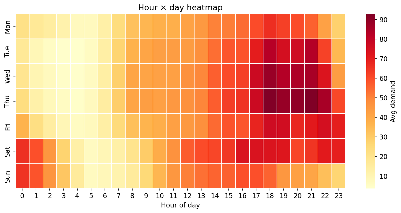
The darkest cells are Thursday through Saturday evenings from 6pm to 10pm. This
interaction between hour and day is the strongest signal in the data. The 7-day same-hour lag feature
captures it directly.
Feature importance
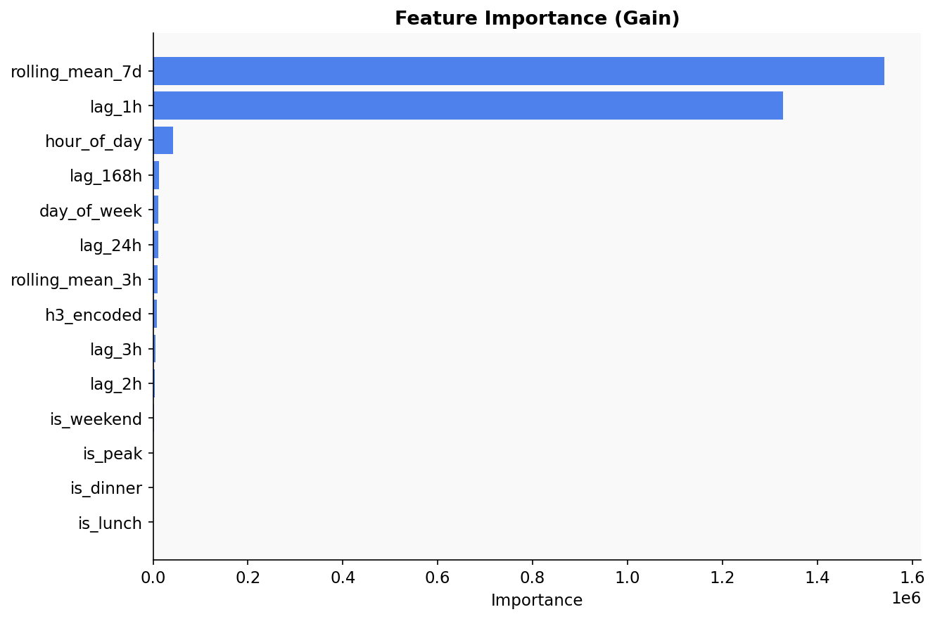
The 7-day rolling average and the 1-hour lag dominate. Last week's demand at this
exact hour in this exact zone is the single best predictor of this hour's demand. Hour of day is a distant
third. The binary flags for lunch, dinner, and weekend contribute almost nothing once the lag features are
present.
Stack
NYC TLC parquet data · H3 spatial indexing · LightGBM · AWS SageMaker Processing Job, Training Job, Model
Registry, Endpoint · Python · pandas · geopandas
View on
GitHub